


Project 2Climate change and global risk assessment
Results of FY 2012
As a way of understanding quantitatively the uncertainty of climate change projections, we tested the “pattern scaling” method. Since this method does not require as high computational resources as global climate models with high spatial-temporal resolution, it has become possible to make future predictions under different emission scenarios which were not possible to make earlier with global climate models. In the figures below, annual average temperatures are shown. This method assumes that with a global mean temperature rise by 1 degree Celsius, the temperature increase at each geographical point will be the same in all the different emission scenarios. However, it has become clear that there are significant differences among emission scenarios, and therefore, attention must be paid when looking at climate impact assessments using the pattern scaling method.
We have also analyzed the possible causes, and showed that there are major differences among emission scenarios with regard to the emissions of sulfate aerosols in the mid-latitudes, and sea ice and the Atlantic Meriodional Overturning Circulation in the high latitudes of the Northern Hemisphere.
In the future we aim to apply this method in various impact assessments, and provide information to facilitate decision making about climate change issues.
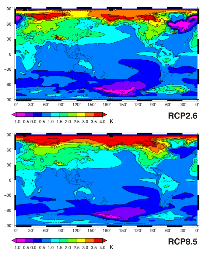
The figure shows the change in surface temperature with a 1 degree C global mean temperature rise in the RCP2.6 and RCP8.5 scenarios. In both scenarios the temperature rise is large in the high latitudes and small in the low latitudes of the Northern Hemisphere. The temperature increase at the same latitude is larger over land than over the ocean. These basic characteristics are almost the same in both scenarios.
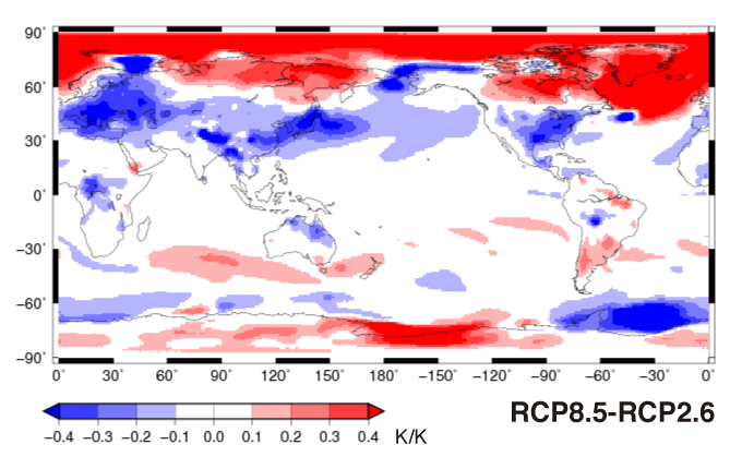
This figure shows the difference in the change of surface temperature with a 1 degree C increase of global mean temperature between the RCP8.5 and RCP2.6 scenarios. There are large differences between the two scenarios in the mid- and high latitudes of the Northern Hemisphere.
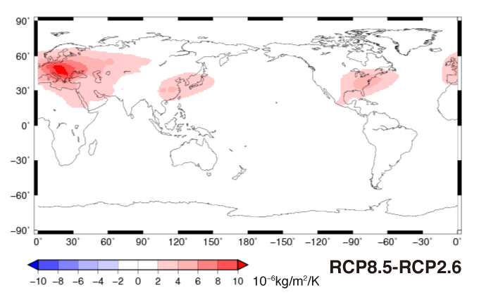
The figure shows the difference in the change of sulfate aerosol in the atmosphere with a 1 degree C increase of global mean temperature between the RCP8.5 and RCP2.6 scenarios. Sulfate aerosols in the atmosphere have a temperature reducing effect by directly or indirectly preventing solar radiation to reach the earth’s surface. According to both scenarios the emissions of sulfate aerosols will be greatly reduced in the future due to technical development, and the size of this reduction is estimated to be about the same by both scenarios. On the other hand, due to the difference in GHG emissions, the increase in global mean temperature greatly differs between the two scenarios. For this reason, in areas with currently large aerosol emissions, there are large differences between the two scenarios with regard to the change in surface temperature with a 1 degree C increase in global mean temperature.
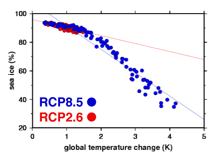
This figure shows the relationship between the ratio of sea ice area over the Arctic and changes in global mean surface air temperature. With the progress of global warming the sea ice over the Arctic is melting, and solar radiation that previously was reflected by the ice, will be absorbed by the sea. As a result, the temperature over the Arctic will further increase, and the more global warming is proceeding, the more the size of the sea ice will decrease. Compared to the RCP 2.6 scenario, the RCP8.5 scenario shows a higher global mean temperature increase, and consequently, since global warming is progressing at an accelerating rate, the RCP8.5 scenario predicts a higher temperature rise over the Arctic with a 1 degree C global mean temperature rise.